Late Night Erlang Test

Fiddling around with Erlang. Wanted to determine the most efficient collection datastructure for membership testing.

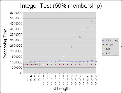
The graph above are the results of that testing. In this test I used integers, although my actual problem does not use integers it did allow me to include the array module in the test.

We can see that using native lists is the faster for small lists. In particular, it is faster to use lists for up to 300 members if your searches are expecting 100% membership rate. Clearly this does not obviously look like a winner, but using lists instead of dicts or arrays could be a good choice for performant mapping. Somthing that was left out for the array test was the fixed size array, this could probably change the performance quite a bit.

Please note that the X-axis is not regularly spaced. I whipped that graph up in open-office calc and its charting capabilities are a bit weak. That sudden climb of the list based solution is not due to some weird threshold but because the test suddenly jumps from incrementing by 100 to incrementing by 500. Oh and the processing time is in milliseconds :)

Here is the Erlang code used for that test.

integer_test(Max) ->
 Iterations = 500000,
 Number_List = lists:seq(1,Max),
 Degree_Of_Error = 1,
 Self_Dict = fun(Number,Number_Dict) ->
                    dict:store(Number,Number,Number_Dict)
             end,
 Test_Dict = lists:foldl(Self_Dict,dict:new(),Number_List),
 Self_Array = fun(Number,Number_Array) ->
                    array:set(Number,Number,Number_Array)
              end,
 Test_Array = lists:foldl(Self_Array,array:new(),Number_List),
 Make_Set = fun(Number,Number_Set) ->
                    sets:add_element(Number,Number_Set)
            end,
 Test_Set = lists:foldl(Make_Set,sets:new(),Number_List),
 Access_Dict = fun() ->
                  Number = random:uniform(Max*Degree_Of_Error),
                  dict:find(Number,Test_Dict)
          end,
 {Time_Dict,_Return_Dict} = timer:tc(util,do_n_times,[Access_Dict,Iterations]),
 Access_Array = fun() ->
                  Number = random:uniform(Max*Degree_Of_Error),
                  array:get(Number,Test_Array)
          end,
 {Time_Array,_Return_Array} = timer:tc(util,do_n_times,[Access_Array,Iterations]),
 Access_Set = fun() ->
                  Number = random:uniform(Max*Degree_Of_Error),
                  sets:is_element(Number,Test_Set)
          end,
 {Time_Set,_Return_Set} = timer:tc(util,do_n_times,[Access_Set,Iterations]),
 Access_List = fun() ->
                  Number = random:uniform(Max*Degree_Of_Error),
                  lists:member(Number,Number_List)
            end,
 {Time_List,_Return_List} = timer:tc(util,do_n_times,[Access_List,Iterations]),
 {Time_Dict,Time_Array,Time_Set,Time_List}.

***UPDATE***

I had some odd results trying to apply this to my sat solver. I managed to track down the reason. lists:member/2 is a BIF. So it has some fast as C implementation. If you try to recreate this test writing your own Erlang member function the behaviour is *very* different.

Dynamic Worksharing

Since we know that we can safely share work by sharing the contents of the workstack, the next step is to organise our processes so they can cooperate and effectively share work and (spectacularly?) speed up our solver.

An Example With two Processes

We will begin in a very simple scenario where we have two processes, process 1 and process 2, available to do work and a single formula as input.

We will consider a process as having two important states.

1. If it has work available, it works
2. If there is no work avaiable, it requests it from another process

We will first start up both of our processes, giving a formula to process 1 allowing it to begin work. Process 1's workstack will initially contain a single entry with the first variable assignment. A single item workstack cannot be shared, so process 2 will have to wait until at least two pieces of work are available.

Process 2 has no work initially, but can request work from process 1. However, there is a chance that this will happen before process 1 has had a chance to produce enough to share. In this case process 1 will respond saying that it has no work to share. Process 2 responds to having it's work request rejected by going to sleep for a while and then requesting work again later. The expectation is that work will be continually generated and will become available in the future. Process 1, meanwhile, will follow the Davis-Putnam algorithm fattening its workstack as it searches for a solution. Now after a brief sleep process 2 can make a second work request and process 1 will most likely have some work to give. After sharing is complete our solver carries on doing twice as much work as before.

This scheme should work for two processes. But clearly, for scalability and our own personal satisfaction, we would like to extend this approach to an arbitrarily large number of cooperating processes.

A Side Note on Termination

It should be noted that in this example we conspicuously neglected an important aspect of our sat solver; termination!

In the case where one process finds a satisfying assignment to the formula being worked on the answer must be communicated back to the caller, while the remaining processes need to be shut down.

In Erlang we can link processes to one another in such a way that terminating one process will cause other linked processes to terminate. This give us a convenient mechanism for halting processes when a satisfying assignment is found. However, in the case where a formula is unsatisfiable this approach is not sufficient.

A formula is known to be unsatisfiable only when every process has an empty workstack. In the two process example we could add some communication that determines whether at least one process has work available. But this approach will not scale well in a many-processes solution. Determining that all work has been exhausted with an arbitrary, or just very large, number of cooperating processes is probably the most exciting and fun aspect of worksharing. It's also a bit fiddly and will have to be covered in a separate post.

Many Processes

In the example of two cooperating processes given above, it was convenient that every process knew about every other process that was working on the same problem. This meant they could easily request work from all other processes and if any was available it would be provided. However, this will not be as effective if we start adding additional processes.

If we allow an arbitrary number of working processes we will need to take a different approach. Linking every process together will prevent scalability as processes spend time and memory dealing with their enormous process lists. For this reason we a better network structure to limit the number of directly linked processes without compromising global communication.

For this purpose we have developed a list network structure for organising processes and allowing (eventual) total communication between all working processes. Working processes are organised in a bi-directionally linked list. The list does not loop so there are always two processes (called the top and bottom respectively) connected to a single process.

When a message, such as a work request, is sent across the network we can easily have the message bounce from process to process along the list until a process with sharable work receives it. If the work request message itself contains the pid (a pid in erlang uniquely identifies a process allowing us to send it messages) of the requesting process we can respond directly without disturbing any other processes.

This does introduce some overhead in having each process mediating messages. But in testing this overhead has been shown to be minimal compared to the work involved in grinding away looking for satisfying assignments to a boolean formula.

As a side note this list structure actually began life as a tree and was later converted into a list. The tree structure has some very charming properties and will be covered in a future post.

Masters, Slaves and Control Issues

The process list network described above is markedly different from the more common master slave architecture used to distribute sat solvers. With our approach it is hoped that we can avoid a strangled master process and facillitate effortless and natural scaling. A lovely dream.

The Work Stack

A Brute Force Approach

As mentioned in a previous post determining the satisfiability of a boolean formula is quite trivial with a brute force algorithm. Here we will look at the brute force algorithm and establish the way that we will talk about solvers 'doing work'.

The most common way to implement a depth first search algorithm is with a stack. For our problem we will be pusing sets of variable assignments onto the stack and pooping them off for processing. We'll illustrate this with a very simple formula

p&q

For formula p&q there are four possible variable assignments.

1. p = true, q = true
   
2. p= true, q = false
3. p = false, q = true
4. p = false, q = false
   

Our search algorithm needs to be able to find each one of those combinations so that we can test the formula for satisfiability.

We begin by selecting a variable, p, at random and pushing it's two possible assignments onto the stack. So our stack looks like:

• p=false
• p=true
  

Each element in the stack will be called a state, because every element in the stack represents a distinct possible (partial) variable assignment for the formula.

Next we will pop the top of the stack, p=true, and select a variable which has not yet been assigned, in this case there is only q. We make two new states with the two possible assignments to q and push them onto the top of the stack. Our stack now looks like:

• p=false, q=false
• p=false, q=true
• p=false

Again we pop the top of the stack. We note that the state we have popped is a complete assignment of the variables in the formula. So we ask does it make the formula true (and therefore satisfiable). By subsituting the assignments for the variables into the formula we get

false & false

which is not true. We must keep searching.

We pop the next value off the stack, p=false, q=true, this is also a full assignment of the variables in the formula. This state does not make the formula true either. We discard these full assignments and keep searching.

We pop the next value off the stack, p=true, this is a partial assignment and so we make two new states with the two possible assignments to q and push them onto the top of the stack. Our stack now looks like:

• p=true, q=false
• p=true, q=true

Popping the top of the stack, p=true, q=false, we find a full assignment which does not make the formula true. We pop the next, and final, element from the stack and find that p=true, q=true makes p&q true and therefore satisfiable.

The Algorithm In Pseudocode

Note that {x,y,z} is the notation for a set and U is the union operator.

F = formula for satisfiability
W = Work stack (initially empty)
S = Current State (set of variable assignments)

Select an unassigned variable V
W.push({V = true})
W.push({V = false})

while (true)
if (W.isEmpty())
return unsatisfiable
else
S = W.pop()
if (isFullAssignment(S,F) and satisfies(S,F))
return satisfiable
else
V = getUnassigned(F,S)
S1 = S U {V = true}
S2 = S U {V = false}
W.push(S1)
W.push(S2)
end

A Problem Shared is a Problem Halved (ignoring overhead)

An Introduction to Parallel Search

Since we know that the work which our sat solver does is contained in a stack we can now take the easy step of parallelising our solver by splitting up the stack and sharing it between two processes.

In this post we will cover this simple procedure and introduce and compare two approaches to parallel programming, namely synchronization (Java) based and message passing (Erlang) based.

The Trivial Act of Sharing Work

The act of splitting the work stack requires a donor process (roughly speaking Erlang has processes where Java has threads) who has work to give and a recipient process who has no work and recieves it from the donor.  Once the work has been shared each process can resume sequential work on their respective workstacks.

Message Passing Parallelism

Previous to this post we haven't mentioned any parallel aspects of our Sat Solver at all. So it seems like a good idea to take this opportunity to introduce Erlang paralellism (usually called message passing parallelism or the Actor model) as it is the core of the implementation of our distributed Sat Solver.  I will be using Java to compare Erlang with a more mainstream approach to parallelism.

In Java, two threads will usually coordinate their behaviour by calling synchronised methods on shared Objects.  For example; Imagine a scenario where threads could to share their workstack with other threads provided there was at least one other thread who had no work to do.  We would probably use a thread pool (like ExecutorService) whose methods would test the current count of working threads and see if there are any available.  These methods must clearly be synchronized to prevent multiple threads attempting to share work simultaneously.

By contrast, in Erlang two processes could not update a shared counter of since all data is immutable.  Instead processes communicate by sending messages to each other.  In this case we could recreate the 'thread pool' we used in the java example by creating a seperate process which accepts messages from workers and launches a new process if this is appropriate.  We should observe that this approach requires the process wishing to share its work to wait for a response from the 'thread pool' process to find out whether or not its work was shared and what work remains after sharing has taken place. 

This Erlang solution is simple to program because it has not tricky synchronisation but it does share with the Java approach one key feature, a single point of communication.  In the Java threads interact by passing through a synchronized block where only one thread may run at a time.  Similarly in Erlang we are passing all of our messages to one process and waiting for a response.  In both cases a large amount of simultaneous work sharing will create performance degrading contention in the java example and fill the mailbox of our 'thread pool' process in Erlang.

It is a very simple modification to the Erlang system to have each process individually track the number of processes currently running and spawn processes directly in order to share work.  This removes the bottleneck but introduces some other oddities which will be discussed in more detail in later posts.

The Standard Algorithm

Davis-Putnam-Logeman-Loveland

The algorithm which is the most popular solution to the satisfiability problem was originally developed by Martin Davis, Hillary Putnam, George Logemann and Donald W. Loveland in 1962. Below I will try to give a simple outline of how this algorithm works which will, hopefully, clarify the design decisions made later.

Satisfaction a Clause at a Time

The search for satisfiability is essentially a search for values assigned to variables in the formula which make the entire formula true. Since we know that our formula is in CNF (see previous post) we can exploit some convenient properties to make it easier to find good assignments.

1. Only one literal needs to be true in a clause for the entire clause to be true
2. When every clause in a formula is true the entire formula is true

Assigning Values

Given the formula:

1: (pV~q)&(~pVqVr)

We can assign the values true or false to either p, q or r.

If we assigned p to true then the literal p is true and ~p is false.

If we assign both r and p to be true then the first clause, (pV~q), is true because p is true. The second clause, (~pVqVr), is true because r is true. Thus the entire formula is true and we know don't even need to try out any assignments for q.

A Two Step Search

The search procedure can be divided into two easy steps. There is actually an extra step described in the original algorithm but is not employed commonly in real world solvers.

1. Unit Propogation - If any clause in the formula contains a single literal whose variable has not been assigned (and all other literals are false) then we know that in order to make that clause true we must make that literal true. These literals are called unit literals. In this step we repeatedly assign values to variables to make any unit literals true.
2. Variable Selection - At this step we select a variable which has not yet been assigned a value and our search tree branches on assigning it true or false.
   

Boolean Formula and Satisfiability

A Quick Introduction to Boolean Logic

The simplest possible Boolean formula contains a single variable.  

1: p

Here p can be either true or false.  When p is true the entire formula is true.  When p is false the formula is false.

Additionally we can negate a variable appearing in a formula.

2: ~p

When p is true ~p is false and vise versa.

From now on we will call a variable appearing in a formula a literal and a negated variable a negative literal.  For example we would say that formula 1 contains a single literal and formula 2 contains a single negative literal.

To build a formula with more than one literal we need some operators.  Boolean formulas have two operators commonly called and and or.  Below I will use the characters & and V for these when writing out formulas.

3: p&q

3 is true only when both p is true and q is true.

4: pVq

4 is true when p is true or q (or both) is true.

We can add parenthesis to a formula having the same effect as parentheses in high school maths.

5: r&(pVq)

5 is true when r is true and either p or q are true. 

Satisfiability

A formula is satisfiable if it is possible to give its variables values which make the entire formula true.

6: p

6 is definitely satisfiable because when we make p true the entire formula is true.

7: ~p

7 is also satisfiable because we can make p false and the formula true.

8: ~pVp

8 is satisfiable, in fact no matter what value we give to p this formula will be true.

9: ~p&p

9 is not satisfiable because there is no way to make p and ~p true at the same time.

Conjunctive Normal Form

A formula is said to be in conjunctive normal form (CNF) it looks like this.

6: (aV~bVc) & (~aVb) & (aVdV~cV~e) & (c) & (cVeV~f)

Each literal is connected by the V operator in a row we will call a clause.  For example the first clause in 6 is (aV~bVc).  Each clause is connected to another clause by the & operator.  For every Boolean formula there is an equivalent (equally satisfiable) formula in CNF.

A formula in CNF is satisfiable if at least one literal from each clause can be made true.

An Easy Problem

Writing a computer program to determine whether or not a Boolean formula is satisfiable is very straight forward.  We can clearly try every possible combination of true and false for every variable in the formula asking at each step whether or not the formula is satisfiable.  Unfortunately if we have n variables there are 2^n possible combinations and we quickly run out of time left in the universe for solving our problem.

Cleverer algorithms have managed to determine satisfiability in times much faster than 2^n, and adding processing power by distributing the computation is a fun next step.

My Fun Project

I have developed the beginnings of a distributed sat solver in Erlang.  This blog is my place to write down my ideas about writing distributed sat-solvers and also describe what I have developed so far.  It is also an open invitation to people who are interested in this kind of software to commment and discuss the development of a distributed sat-solver in Erlang.

I became interested in developing parallel applications after finishing a CPU heavy graph algorithm and noticing that the program was running for one hour at 50% CPU!  Clearly I would have to rewrite alot of code just to use all the computing power available on my old inspiron laptop.  After reading up on Java threading (I'm a Java developer by day) I stumbled on a blog entry talking about concurrency minus the tricky shared state. It was also a vicious tirade about the ignorance of Java developers.  The author recommended Erlang and I like the idea of concurrent programming without the goto-like hassles of synchronisation.

I picked the boolean satisfiability problem because depth first search doesn't obviously lend itself to easily balanced work sharing. I started coding in a language I barely understood.  It doesn't get much better than this.